Bank capital-at-risk: measuring the impact of cyclical systemic risk on future bank losses
Cyclical systemic risk tends to build up well ahead of financial crises and is measured best by credit and asset price dynamics. This article shows that high levels of cyclical systemic risk lead to large downside risks to the bank-level return on assets three to five years ahead. Hence, exuberant credit and asset price dynamics tend to increase considerably the likelihood of large future bank losses. Given the tight link between bank losses and reductions in bank capital, the results presented in this article can be used to quantify the level of “Bank capital-at-risk” (BCaR) for a banking system. BCaR is a useful tool for macroprudential policy makers as it helps to quantify how much additional bank resilience could be needed if imbalances unwind and systemic risk materialises.
1 Introduction
Financial crises are rare events, but when they occur they tend to go hand in hand with large declines in output and, oftentimes, heavy losses for banks. For example, various studies (Lo Duca et al., 2017; Laeven and Valencia, 2012) have shown that cumulative GDP losses during past financial crises amounted on average to 8‑20% of annual GDP. In addition, as shown in Lang and Forletta (2019) and further below in Section 3, the banking sector return on assets (ROA) in EU countries tended to be considerably lower during past financial crises than during normal or pre-crisis times. In particular, losses of at least 0.6% of total assets were observed in more than one quarter of all financial crisis years over the past 40 years.
With this background in mind, this article studies the impact of cyclical systemic risk on future bank profitability for a large panel of EU banks. The analysis builds on recent advances in the literature on measuring cyclical systemic risk and its impact on the real economy. First, we use the domestic cyclical systemic risk indicator (d‑SRI) proposed by Lang et al. (2019) as our time-varying cyclical systemic risk measure. The d‑SRI is a tractable and transparent country-level measure of the financial cycle that increases, on average, around five years before the onset of financial crises and that contains information about the likelihood and the severity of financial crises in terms of GDP losses. Second, we employ quantile local projections as proposed by Adrian et al. (2019) to quantify the impact of the d‑SRI on tails of the bank-level ROA distribution over horizons of one to six years ahead.
The main result of the analysis is that high cyclical systemic risk leads to large downside risks to future bank profitability and therefore to bank capital. In particular, we show that the impact of cyclical systemic risk on the left tail of the future bank-level ROA distribution is an order of magnitude larger than that on the median. The estimated impact of a one-unit d‑SRI on the lower fifth percentile of the conditional pre-tax ROA distribution is in the range of ‑1.1 to ‑1.8 percentage points for horizons of three to five years ahead. The corresponding numbers for the impact on the median are in the range of ‑0.15 to ‑0.25 percentage points at the three to five year horizon. These estimates illustrate that high cyclical systemic risk shifts the entire future bank-level ROA distribution downward, but its impact is by far the highest on the left tail of the future ROA distribution. Given that negative profits directly reduce bank capital ratios, the method can be used to quantify the level of future “Bank capital-at-risk” for a given banking system, akin to the concept of “Growth-at-risk” developed by Adrian et al. (2016). This measure can be useful to inform macroprudential policy.
The remainder of this article is structured as follows: Section 2 briefly discusses the d‑SRI, which is our measure of cyclical systemic risk. Section 3 provides a descriptive overview of the relationship between banking sector losses and cyclical systemic risk in euro area countries over the past 40 years. Section 4 outlines the empirical methodology to identify the impact of cyclical systemic risk on the future bank-level ROA distribution. Section 5 provides details regarding the main empirical finding that high cyclical systemic risk leads to large downside risks to future bank profitability. Finally, Section 6 illustrates how the method can be used to quantify the level of future “Bank capital-at-risk” for a given banking system. Section 7 concludes.
2 Measuring cyclical systemic risk in euro area countries
An emerging consensus in the academic literature is that cyclical systemic risk builds up gradually and well in advance of financial crises. Various papers have shown that credit cycle measures or composite financial cycle measures that combine credit and asset prices display cycle lengths of around 15‑20 years and are among the most useful indicators to assess the probability of financial crises with a lead time of several years.[2] In addition, credit or composite cycle measures have been shown to contain advance information about the severity of financial crises and recessions measured in terms of real GDP declines.[3]
For our analysis we use the domestic cyclical systemic risk indicator (d‑SRI), which was developed at the ECB as a measure of the financial cycle.[4] The d‑SRI is a broad-based country-level indicator that captures the build-up of cyclical systemic risk emanating from domestic credit, real estate markets, asset prices, and external imbalances. It is constructed as a weighted average of six well-performing early warning indicators for financial crises, after they are normalised to the same scale. Indicator normalisation is performed by subtracting the median and dividing by the standard deviation of the pooled indicator distribution across countries and time. Indicator weights are chosen to maximise the early warning performance of the d‑SRI for domestically-driven systemic financial crises with a lead time of 12‑5 quarters.[5]
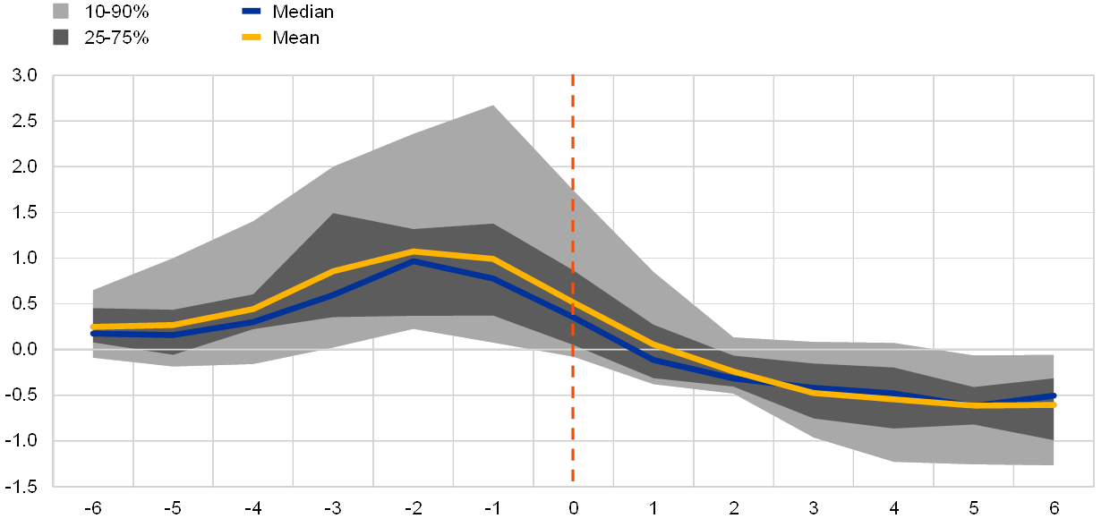
As shown in Lang et al. (2019), the d‑SRI contains valuable information about the likelihood and severity of financial crises with a lead time of several years. For example, Chart 1 illustrates that the d‑SRI tends to increase, on average, around five years before the onset of financial crises. In addition, model estimates suggest that the d‑SRI has significant predictive power for large declines in real GDP growth three to four years down the line, as it precedes shifts in the entire distribution of future real GDP growth and particularly of its left tail (“Growth-at-risk”).
Chart 1
The d‑SRI, which is a useful measure of cyclical systemic risk in euro area countries, starts to increase on average around five years before financial crises
d‑SRI distribution across euro area countries before past financial crises
(x-axis: years before/after financial crises; y-axis: d‑SRI value)
Sources: Data from Lang et al. (2019) and Lo Duca et al. (2017). The chart is taken from Lang and Forletta (2019).
Notes: The chart shows the mean, median, interquartile range and 90‑10 percentile range across 22 EU countries (euro area countries, Denmark, Sweden, and the United Kingdom) during the six years before and after the onset of systemic financial crises. The dating of systemic financial crises in the chart is based on the ECB/ESRB crises database described in Lo Duca et al. (2017). Purely foreign-induced crises are excluded. The chart is based on 21 systemic crisis events in total. 7 of these crises occurred before the onset of the global financial crisis in 2007.
3 Cyclical systemic risk and bank losses over the last 40 years
There are various channels through which the build-up of cyclical systemic risk can affect future bank profitability and lead to large banking sector losses. First, macro-financial imbalances (e.g. high leverage and asset price overvaluation) can lead to direct credit losses for banks once a negative shock hits and defaults increase due to the fall in asset prices and tighter borrowing constraints. Second, an excessive build-up of leverage in the non-financial private sector can imply large deleveraging needs once borrowing constraints tighten in a crisis situation, which can exert large downward pressure on credit growth and hence on the business volumes of banks. Third, abrupt adjustments of asset price overvaluations can cause losses in banks' trading portfolios. Fourth, indirect negative feedback loops between tighter borrowing constraints, falling asset prices, and reduced economic activity can cause further credit losses for banks. This list of transmission channels between the build-up of cyclical systemic risk and future bank profitability is by no means exhaustive, but it illustrates that there are many relevant channels.
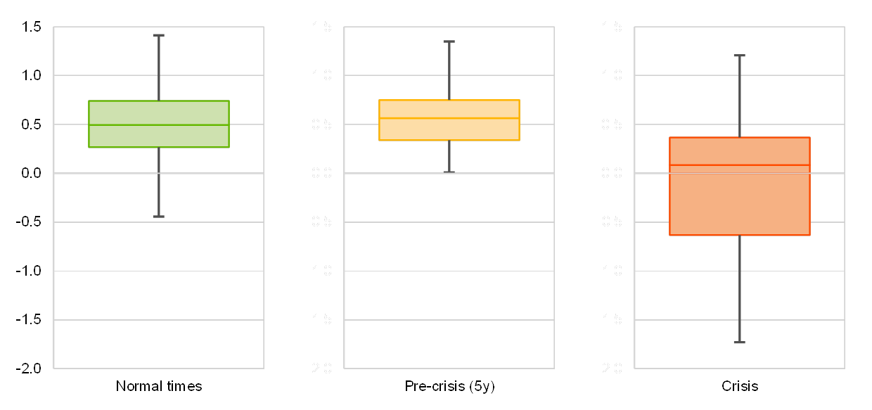
Indeed, over the past 40 years the banking sector ROA in euro area countries was much lower during financial crisis years than in normal times. For example, as shown in Chart 2, the median banking sector ROA during normal or pre-crisis years tended to be close to 0.5%, whereas the median ROA during financial crisis years stood close to 0%. In addition, while aggregate banking sector losses are extremely rare during normal times, losses of at least 0.6% of total assets materialised in more than one quarter of all financial crisis years. Cumulative losses were even larger and amounted to at least 1.5% of total assets during half of the systemic financial crises in EU countries over the last 40 years (Calculations are based on the same data, however the chart is not shown here but contained in Lang and Forletta (2019)).
Chart 2
The banking sector ROA tended to be much lower during financial crises than in normal times and in many instances large banking sector losses materialised
Conditional distributions of the annual banking sector ROA in euro area countries
(x-axis: state of the economy; y-axis: banking sector ROA)
Sources: OECD, CBD2, authors’ calculations. The chart is taken from Lang and Forletta (2019).
Notes: The underlying data covers a panel of 22 countries (euro area countries, Denmark, Sweden, and the United Kingdom) since 1980. The number of countries with data varies over time: 1980 (7 countries), 1985 (10 countries), 1990 (14 countries), 1996 (17 countries), 2008 (22 countries). The dating of systemic financial crises in the chart is based on the ECB/ESRB EU crises database described in Lo Duca et al. (2017). Purely foreign-induced crises are excluded. The chart is based on 21 systemic crisis events in total. Seven of these crises occurred before the onset of the global financial crisis. The three lines that divide the coloured box areas into two ranges represent the 25th, 50th and 75th percentiles, while the other two lines represent the lower and upper adjacent values.
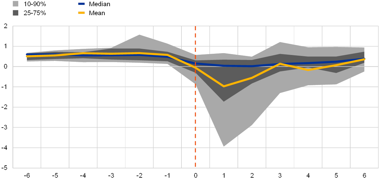
Visual comparison of the d‑SRI and ROA around financial crises suggests that increases in cyclical systemic risk precede declines in bank profitability. This lead-lag pattern is clearly visible when comparing Charts 1 and 3. For example, the d‑SRI tends to increase continuously during pre-crisis years, reaching a peak between one and two years ahead of the materialisation of a financial crisis (see Chart 1). In contrast to this, the banking sector ROA does not move much ahead of financial crises, but tends to fall significantly following the onset of a crisis (see Chart 3). There is usually a protracted fall in banking sector profitability following the start of a financial crisis, and only a gradual rebound to pre-crisis levels after many years. These lead-lag patterns motivate our empirical analysis of the impact of cyclical systemic risk on future bank profitability and in particular on the left tail of the profitability distribution.
Chart 3
The start of a financial crisis is usually followed by a prolonged decline and eventual rebound in the banking sector ROA
Banking sector ROA distribution across euro area countries before past financial crises
(x-axis: years before/after financial crises; y-axis: banking sector ROA)
Sources: OECD, CBD2, Lo Duca et al. (2017), authors' calculations. The chart is taken from Lang and Forletta (2019).
Notes: The chart shows the mean, median, interquartile range and 90‑10 percentile range across 22 EU countries (euro area countries, Denmark, Sweden, and the United Kingdom) during the six years before and after the onset of systemic financial crises. The dating of systemic financial crises in the chart is based on the ECB/ESRB crises database described in Lo Duca et al. (2017). Purely foreign-induced crises are excluded. The chart is based on 21 systemic crisis events in total. Seven of these crises occurred before the onset of the global financial crisis in 2007.
4 Overview of the empirical methodology and dataset
To study the impact of the d‑SRI on future bank profitability we make use of the “Growth-at-risk” methodology recently proposed by Adrian et al. (2016). In particular, we employ quantile local projections on a bank-level dataset to quantify the impact of the d‑SRI on the lower left tail of the bank-level ROA distribution over horizons of one to six years ahead. The advantage of using quantile regressions compared to linear regressions is that they allow for heterogeneous effects of the d‑SRI in different parts of the bank profitability distribution. In addition, the local projections framework proposed by Jordà (2005) allows to estimate such effects for different prediction horizons in a flexible way with the possibility to account for a rich set of control variables. The focus on the lower left tail of the bank profitability distribution helps shed light on potential losses due to cyclical systemic risk and is therefore of high relevance for macroprudential policy.
Our model links future values of the bank-level pre-tax ROA to current values of the d‑SRI, bank- and country-specific controls, as well as country and time fixed effects. In particular, we control for the following bank-specific variables which could affect future bank profitability: the net interest margin, the cost-to-income ratio, the ratio of impairments to total assets, the share of loans in total assets, the average risk-weight, the leverage ratio, the Tier1 capital ratio, the log of total assets, and the current pre-tax ROA. We also control for a number of country-level banking sector and macro-financial factors: the bank credit-to-GDP ratio, the Herfindahl-Hirschman Index based on total bank assets, the annual real GDP growth rate, the annual inflation rate, the three-month Euribor, the slope of the yield curve (difference between the ten-year government bond yield and Euribor), the annual growth rate of equity prices and the annual growth rate of real estate prices.
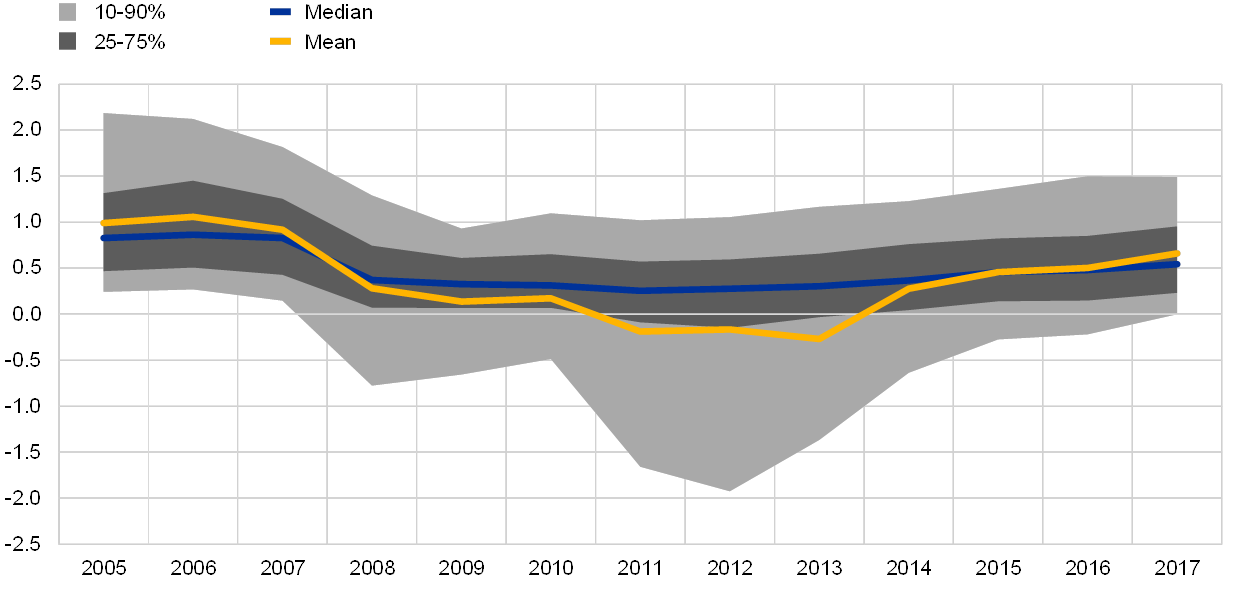
The model is estimated using a large representative panel dataset covering more than 450 banks from 22 EU countries between 2005 and 2017. The annual dataset was sourced from SNL Financial and covers banks from all euro area countries, Denmark, Sweden, and the United Kingdom. The bank sample was chosen to ensure representativeness of country-level aggregate banking sectors. Chart 4 shows the evolution over time of the pre-tax ROA distribution across the banks in our sample. A clear downward shift is visible after the start of the global financial crisis in 2008, particularly of the lower left tail of the distribution. The country-level control variables were sourced from the ECB Statistical Data Warehouse and the d‑SRI was taken from Lang et al. (2019).
Chart 4
The distribution of the pre-tax ROA across euro area banks shifted downward considerably between 2008 and 2013, following the global financial crisis
Evolution of the distribution of the pre-tax ROA across banks
(y-axis: pre-tax return on assets in percent; x-axis: years)
Sources: SNL Financial, authors’ calculations. The chart is taken from Lang and Forletta (2019).
Notes: The chart shows the mean, median, interquartile range and 90‑10 percentile range of bank-level pre-tax ROA across an unbalanced panel of 473 banks from 22 EU countries (euro area countries, Denmark, Sweden, and the United Kingdom) during the years 2005 to 2017. The sample of banks was selected to be representative of the aggregate country-level banking sectors.
Compared to the existing “Growth-at-risk” literature, our approach provides three distinct innovations that make it useful for macroprudential policy. First, we employ bank-level microdata instead of aggregate country-level data. The availability of a large cross-section of banks for each country-level financial crisis episode should considerably increase the power to identify the impact of rare aggregate shocks. Second, we focus our analysis on bank profitability as the outcome variable instead of on real GDP, as for example in Adrian et al. (2016), Adrian et al. (2018), Aikman et al. (2018), and Lang et al. (2019). As negative bank profits (losses) can be directly translated into bank capital reductions, our method can inform the calibration of macroprudential capital buffers for the banking system. Third, we focus on the impact of cyclical systemic risk (the d‑SRI) instead of financial conditions. As shown below, the much longer lead time of the d‑SRI of three to five years should allow sufficient time to enact mitigating macroprudential policy measures, once risks are identified.
5 Cyclical systemic risk and downside risks to bank profitability
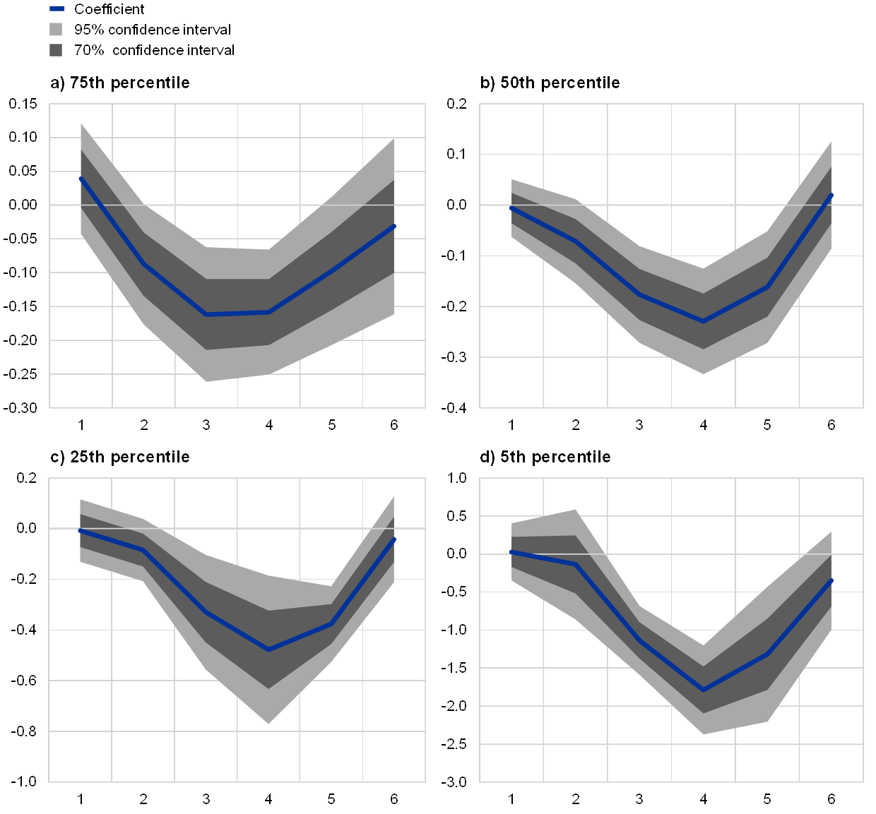
Our empirical results show that high cyclical systemic risk today leads to large downside risks to bank profitability in the following three to five years. In particular, high values of the d‑SRI shift the entire future bank-level ROA distribution downward at these horizons. However, its impact on the left tail of the future bank-level ROA distribution is an order of magnitude larger than that on the median. This can be seen from Chart 5, which shows the estimated impact of the d‑SRI, our measure of cyclical systemic risk, on different quantiles of the future bank-level pre-tax ROA distribution for horizons of one to six years ahead.
For example, a one-unit d‑SRI value leads to a drop in the median bank-level pre-tax ROA of around ‑0.25 percentage points four years down the road. For horizons of three and five years ahead, the estimated impact of a one-unit d‑SRI value on median bank profitability is around ‑0.15 percentage points (see Panel B in Chart 5). Given that the average d‑SRI value ahead of past financial crises is around one (see Chart 1), these estimated effects can be interpreted as the impact on median bank profitability during the average financial crisis. Considering that the unconditional median pre-tax ROA in the data is 0.44%, these estimated negative effects are economically relevant, while also being statistically significant for horizons of three to five years ahead. For horizons of one to two years ahead and horizons beyond five years, the estimated impact is not statistically significant (see Panel B in Chart 5).
Most importantly, the negative impact of the d‑SRI on the lower left tail of the profitability distribution is an order of magnitude larger than that on the median. For example, as shown in Panel D in Chart 5, the estimated impact of a one-unit d‑SRI value on the lower 5th percentile of the pre-tax ROA distribution at the three to five year horizon is between ‑1.1 and ‑1.8 percentage points. This compares to an estimated impact for the three to five year horizon in the range of ‑0.15 to ‑0.25 for the median, and an estimated impact in the range of ‑0.1 to ‑0.15 for the 75th percentile (see Panels A and B in Chart 5) . These figures illustrate the considerable heterogeneity in the impact of cyclical systemic risk on different bank profitability quantiles, which would be concealed by linear local projections.
Chart 5
High cyclical systemic risk today leads to large downside risks to bank profitability in the following three to five years, with considerable non-linearities present
Estimated impact of the d‑SRI on different quantiles of the pre-tax ROA distribution
(y-axis: impact of the d‑SRI on pre-tax ROA in percentage points; x-axis: prediction horizon in years)
Sources: Authors’ calculations based on SNL Financial and other data sources. The chart is taken from Lang and Forletta (2019).
Notes: The charts show the responses of different quantiles of the pre-tax ROA distribution to a one-unit value of d‑SRI for horizons of one to six years ahead. The blue lines plot the estimated coefficients for the d‑SRI from the quantile local projections. Grey shaded areas represent the one and two standard error bounds based on robust standard errors clustered at the bank level. The quantile regressions are estimated on an unbalanced panel of 473 EU banks covering the period 2005 to 2017. All specifications control for bank-, banking sector- and country-specific characteristics as well as country and year fixed effects.
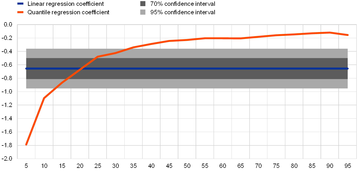
The impact of the d‑SRI on all ROA quantiles above the median is similar in magnitude, while below the median the impact becomes increasingly negative. As shown in Chart 6 for the four-year horizon, the estimated impact on quantiles above the median is in the range of ‑0.15 to ‑0.25. Large non-linearity in the impact of cyclical systemic risk on the bank-level pre-tax ROA distribution mainly starts to kick in for the 25th percentile and lower quantiles. The estimated impact on lower quantiles (5th and 10th) and upper quantiles (95th and 90th) both lie outside the two standard error bounds of the estimated average impact from linear local projections (see Chart 6). This illustrates the value added from running quantile local projections instead of a linear model. It also highlights the disproportionate impact of cyclical systemic risk on downside risks to bank profitability.
Chart 6
The negative impact of the d‑SRI on the lower left tail of the profitability distribution is an order of magnitude larger than that on the median
Estimated impact of the d‑SRI on different pre-tax ROA quantiles four years ahead
(y-axis: impact of the d‑SRI on pre-tax ROA in percentage points; x-axis: quantiles)
Sources: Lang et al. (2019), SNL Financial, ECB, authors’ calculations. The chart is taken from Lang and Forletta (2019).
Notes: The chart shows the response of different quantiles of the bank-level pre-tax ROA distribution to a one-unit value of d‑SRI today at a four-year ahead horizon, compared to the estimate of the average impact. The red line plots the coefficients from the various quantile local projections. The blue line represents the coefficient from a linear local projection model, where the grey shaded areas represent the one and two standard error bounds based on robust standard errors clustered at the bank level. The regressions are estimated on an unbalanced panel of 473 EU banks covering the period 2005 to 2017. All specifications control for bank-, banking sector- and country-specific characteristics as well as country and year fixed effects.
The main empirical results regarding the link between cyclical systemic risk and future bank profitability are qualitatively and quantitatively robust. For example, as shown in Lang and Forletta (2019), the findings of a long lead time of the d‑SRI and the much bigger impact on the left tail of the bank profitability distribution than on the median are both robust to changes in the country sample and the underlying bank sample.
6 Measuring bank capital-at-risk
As negative profits directly reduce bank capital ratios, our results can be used to quantify the level of “Bank capital-at-risk” (BCaR) for a banking sector. The concept of BCaR is similar to the concept of “Growth-at-risk” developed by Adrian et al. (2016) and focuses on future downside risks as represented by the estimated lower 5th quantiles of the model. To translate our estimates based on pre-tax ROA into effects on bank capital ratios, results first need to be divided by the bank-level risk-weight density, which is on average around 50%. The banking sector BCaR is then obtained by aggregating the rescaled lower 5th quantiles of the predicted bank-level ROA distributions across all banks, where aggregation weights are given by the relative size of each bank (in terms of total assets). Our preferred BCaR horizon is four years ahead, as this leaves sufficient time for mitigating macroprudential policy action and the impact of the d‑SRI on bank profitability is also highest at this horizon.
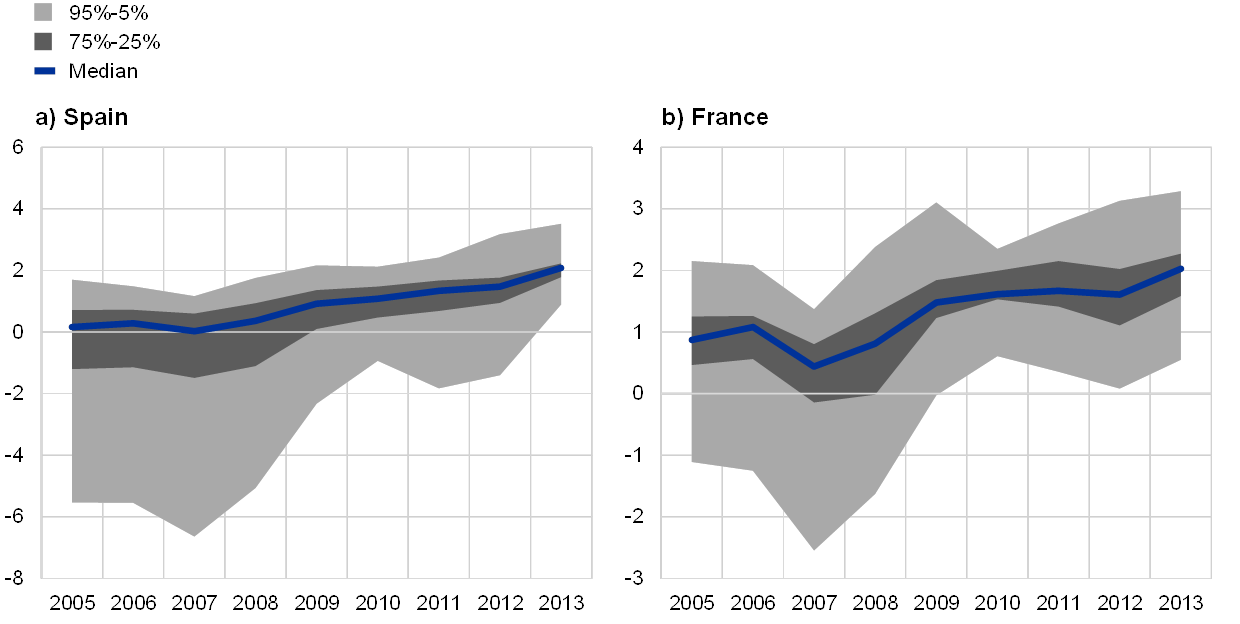
The potential usefulness of the approach is illustrated in Chart 7, which shows the evolution of the four-year-ahead BCaR for Spain and France from 2005‑13. The BCaR for Spain in 2005 of more than ‑5% already indicated significant future downside risks to bank capital ratios. The BCaR for Spain increased further to more than ‑6% in 2007 and then began to decrease gradually in subsequent years. Chart 7 further shows that even the 25th percentile of the conditional density of risk to bank capital for Spain was negative between 2005 and 2008. As a comparison, the BCaR for France was also negative in 2005, albeit at a lower level of around ‑1%, and it peaked in 2007 at around ‑2.5%. However, the 25th percentile of the conditional density of risk to bank capital for France remained above or close to zero throughout the period. Hence, BCaR would have clearly distinguished the levels of risk to bank capital in Spain and France ahead of the global financial crisis.
Chart 7
The proposed BCaR measure would have clearly distinguished the levels of risk to bank capital in Spain and France ahead of the global financial crisis
Four-year-ahead predicted distribution of changes in banking sector capital ratios for Spain and France. “Bank capital-at-risk” (BCaR) is equal to the lower 5th percentile
(y-axis: quantiles of predicted changes in the banking sector capital ratio four-years ahead; x-axis: years)
Sources: Lang et al. (2019), SNL Financial, ECB, authors’ calculations. The chart is taken from Lang and Forletta (2019).
Notes: The charts show the four-year-ahead predicted distributions of changes in banking sector capital ratios for Spain and France based on the model. BCaR is equal to the lower 5th percentile of this predicted distribution. BCaR is computed as a weighted average of the bank-level lower 5th percentiles of the conditional pre-tax ROA distributions after converting them into units of regulatory capital ratios by using bank-level average risk weights. The four-year prediction horizon implies that the density plotted in 2005 is the one predicted for 2009. The blue line is the prediction for the median banking sector capital ratio change, while light and dark grey areas are the 95th–5th percentile range and interquartile range respectively.
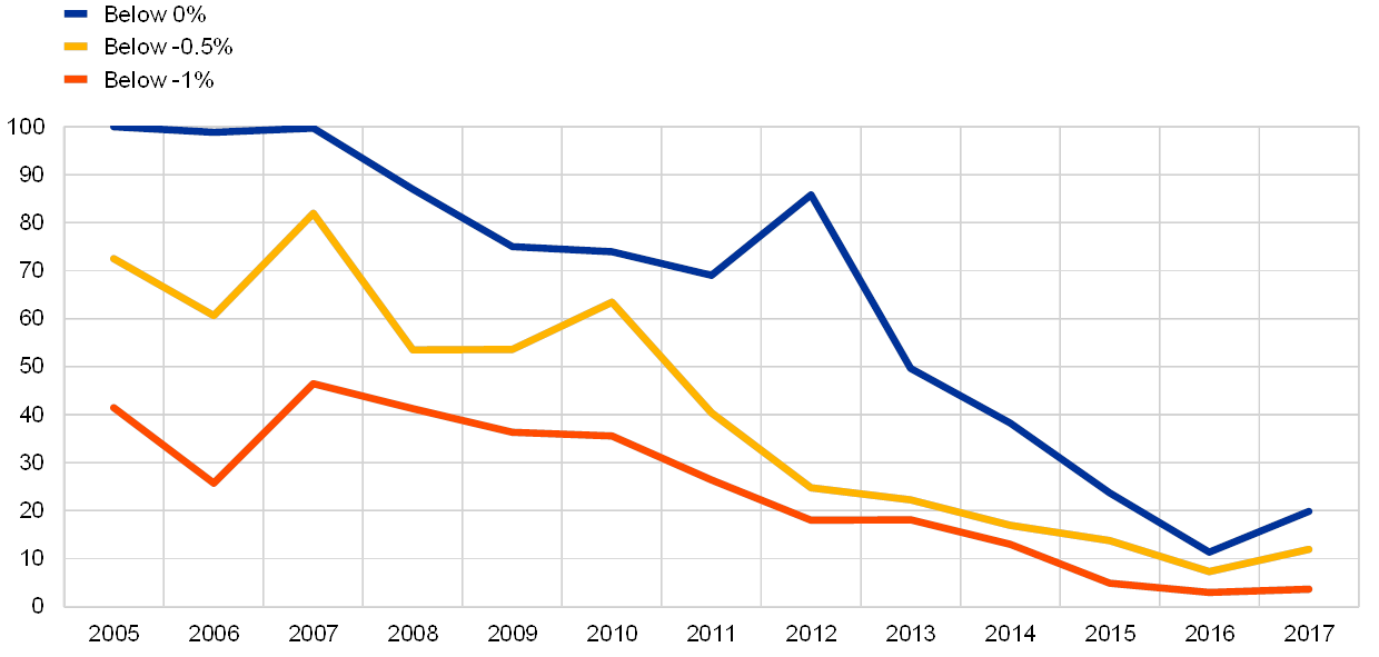
Our framework based on microdata also allows us to derive aggregate country-level risk measures that take into account bank-level heterogeneity. For example, from a policy perspective the main interest could be in banks that are expected to have losses above a given threshold with at least a 5% probability. Hence, computing the asset share held by such banks can shed additional light on vulnerabilities in the banking sector. We call this measure “Share of Vulnerable Banks” (SVB). Chart 8 shows that the four-year-ahead SVB in the euro area was around 40% between 2005 and 2010, based on a loss threshold of ‑1% of total assets. It decreased steadily since then to slightly above zero in 2017. For a loss threshold of ‑0.5%, the respective euro area SVB values were between 60% and 80% during the period 2005‑10, and declined to around 10% by the end of 2017.
Chart 8
e share of assets held by banks predicted to make losses with at least a 5% probability has declined substantially since the start of the global financial crisis
Share of vulnerable bank assets in the euro area at the four-year-ahead horizon
(y-axis: percentage of total bank assets; x-axis: years)
Sources: Lang et al. (2019), SNL Financial, ECB, authors’ calculations. The chart is taken from Lang and Forletta (2019).
Notes: The chart shows the asset share of banks whose predicted four-year-ahead conditional 5th ROA quantile is below a certain threshold (SVB). For example, the values plotted for 2005 are the predicted SVBs for 2009, conditional on information available in 2005. Euro area SVB is plotted for three different ROA thresholds: 0, ‑0.5, and ‑1.0.
7 Conclusion
This article has shown that high levels of cyclical systemic risk lead to large downside risks to bank profitability with a lead time of three to five years. For our analysis we used the ECB’s domestic cyclical systemic risk indicator (d‑SRI), which is a broad-based composite indicator capturing risks from domestic credit, real estate markets, asset prices, and external imbalances.[6] Based on data for more than 450 EU banks for the period 2005 to 2017 we showed that high values of the d‑SRI shift the entire future bank-level profitability distribution downward, but the negative impact on the left tail of the future profitability distribution is by far the largest. For d‑SRI values that typically precede the onset of financial crises, the estimated impact on the lower 5th percentile of the pre-tax ROA distribution is ‑1.8 percentage points at the four year horizon. This impact is economically highly significant compared to the average pre-tax ROA of 0.44% in our dataset.
Given the tight link between negative profits and reductions in bank capital, our results can be used to quantify the level of “Bank capital-at-risk” (BCaR). The concept of BCaR is similar to the concept of “Growth-at-risk” developed by Adrian et al. (2016) and focuses on future downside risks to bank capital. The banking sector BCaR is obtained by aggregating the lower 5th percentiles of the predicted bank-level ROA distributions across all banks, where aggregation weights are given by the relative size of each bank and taking into account the average risk-weight. BCaR is a useful tool for macroprudential policy makers as it helps to quantify how much additional bank resilience could be needed if macro-financial imbalances unwind and systemic risk materialises. As shown in this article, BCaR would have clearly distinguished the levels of risk to bank capital in Spain and France ahead of the global financial crisis.
Compared to the existing “Growth-at-risk” literature, “Bank capital-at-risk” features three innovations that make it useful for macroprudential policy. First, it focuses on downside risks to bank capital instead of real GDP, which can help inform the calibration of macroprudential capital buffers for the banking system. Second, it is derived from bank microdata instead of country-level aggregates, which allows taking into account bank heterogeneity. Third, BCaR uses the d‑SRI – our preferred measure of cyclical systemic risk – as the driver of variations in tail risk, whereas “Growth-at-risk” has mainly focused on financial conditions indices. The lead time of the d‑SRI for changes in BCaR is mainly between three and five years ahead, while the lead time of financial conditions indices for “Growth-at-risk” is mainly between one and four quarters ahead. The long lead time of the d‑SRI and the associated BCaR measure is an important feature to allow for potential mitigating macroprudential policy action if risks are identified.
8 References
Adrian, T., Boyarchenko, N. and Giannone, D. (2016), “Vulnerable Growth”, Staff Report No 794, Federal Reserve Bank of New York.
Adrian, T., Grinberg, F., Liang, N. and Malik, S. (2018), “The Term Structure of Growth-at-Risk”, IMF Working Papers, No 18/180, International Monetary Fund.
Aikman, D., Bridges, J., Burgess, S., Galletly, R., Levina, I., O’Neill, C. and Varadi, A. (2018), “Measuring risks to UK financial stability”, Bank of England working papers, No 738, Bank of England.
Aikman, D., Haldane, A. and Nelson, B. (2015), “Curbing the Credit Cycle”, The Economic Journal, Vol. 125, No 585), pp. 1072‑1109.
Borio, C. and Drehmann, M. (2009), “Assessing the risk of banking crises – revisited” Technical report, Bank for International Settlements.
Borio, C. and Lowe, P. (2002), “Asset prices, financial and monetary stability: exploring the nexus”, BIS Working Papers, No 114, Bank for International Settlements.
Bridges, J., Jackson, C. and McGregor, D. (2017), “Down in the slumps: the role of credit in five decades of recessions”, Bank of England working papers, No 659, Bank of England.
Detken, C., Weeken, O., Alessi, L., Bonfim, D., Boucinha, M.M., Castro, C., Frontczak, S., Giordana, G., Giese, J., Jahn, N., Kakes, J., Klaus, B., Lang, J.H., Puzanova, N. and Welz, P. (2014), “Operationalising the countercyclical capital buffer: indicator selection, threshold identification and calibration options”, ESRB Occasional Paper Series, No 5, European Systemic Risk Board.
Drehmann, M., Borio, C. and Tsatsaronis, K. (2012), “Characterising the financial cycle: don’t lose sight of the medium term!”, BIS Working Papers, No 380, Bank for International Settlements.
Jordà, Ò. (2005), “Estimation and Inference of Impulse Responses by Local Projections”, The American Economic Review, Vol. 95, No 1, pp. 161‑182.
Jordà, Ò, Schularick, M. and Taylor, A.M. (2013), “When Credit Bites Back”, Journal of Money, Credit and Banking, Vol. 45, No s2, pp. 3‑28.
Laeven, L. and Valencia, F. (2012), “Systemic Banking Crises Database: An Update”, IMF Working Papers, No 12/163, International Monetary Fund.
Lang, J.H. and Forletta, M. (2019), “Cyclical systemic risk and downside risks to bank profitability”, Working Paper Series, forthcoming, ECB.
Lang, J.H., Izzo, C., Fahr, S., and Ruzicka, J. (2019), “Anticipating the bust: a new cyclical systemic risk indicator to assess the likelihood and severity of financial crises”, Occasional Paper Series, No 219, European Central Bank.
Lo Duca, M., Koban, A., Basten, M., Bengtsson, E., Klaus, B., Kusmierczyk, P., Lang, J.H., Detken, C. and Peltonen, T. (2017), “A new database for financial crises in European countries”, Occasional Paper Series, No 194, European Central Bank.
Rünstler, G. and Vlekke, M. (2016), “Business, housing and credit cycles”, Working Paper Series, No 1915, European Central Bank.
Schularick, M. and Taylor, A.M. (2012), “Credit Booms Gone Bust: Monetary Policy, Leverage Cycles and Financial Crises, 1870‑2008”, The American Economic Review, Vol. 102, No 2, pp. 1029‑61.
Schüler, Y., Hiebert, P.P. and Peltonen, T.A. (2015), “Characterising the financial cycle: a multivariate and time-varying approach”, Working Paper Series, No 1846, European Central Bank.
- The exposition and results contained in this article are based on Lang, J.H. and Forletta, M. (2019), “Cyclical systemic risk and downside risks to bank profitability”, ECB Working Paper Series, forthcoming.
- See for example Borio and Lowe (2002), Aikman et al. (2015), Borio and Drehmann (2009), Detken et al. (2014), Schularick and Taylor (2012), Drehmann et al. (2012), Schüler et al. (2015), Rünstler and Vlekke (2016), Aikman et al. (2018), and Lang et al. (2019).
- See for example Jordà et al. (2013), Bridges et al. (2017), Aikman et al. (2018), and Lang et al. (2019).
- See Lang et al. (2019) for details on how the d‑SRI was constructed and its performance for predicting the likelihood and severity of financial crises in euro area countries with a lead time of several years.
- Formally, the d‑SRI is defined as follows: . The 6 underlying early warning indicators and optimal weights are: the 2‑year bank credit-to-GDP change (36%), the current account to GDP balance (20%), the 3‑year residential real estate price-to-income ratio change (17%), the 3‑year real equity price growth (17%), the 2‑year debt service ratio change (5%), and the 2‑year real total credit growth (5%).
- See Lang et al. (2019) for details on how the d‑SRI was constructed and its performance for predicting the likelihood and severity of financial crises in euro area countries with a lead time of several years.


